Jane Street's Robot Baseball Puzzle: Markov Games and Golden Section Search
- Modeling a Single-Turn Zero-Sum Game
- Modeling a Simultaneous-Move Markov Game
- Visualizing the Value and Reach Probability as Functions of p
- Black Box Search and Solving the Puzzle
Recently, I have been enjoying solving Jane Street’s backlog of puzzles. Last night, I solved Robot Baseball from October 2025. This post is my write-up of the math I learned while solving it, so if you haven’t already, take a second to read the puzzle!
In brief, Robot Baseball is a Markov game. Its states are numbers of balls and strikes. The game ends when balls=4 or strikes=3. To find the Nash equilibria at each state, we need to first model the terminal states and then use backward induction to solve each subgame equilibrium until we have found an equilibrium for each possible state.
The catch is that if the pitcher throws a strike and the batter swings, the batter hits with probability \(p\) and misses with probability \(1 - p\). We want to optimize \(p\) to maximize our odds of reaching \((\text{balls}=3, \text{strikes}=2)\). The players’ payoffs at each step and their equilibrium strategies are therefore functions of \(p\). This is straightforward symbolically when we are calculating the equilibrium for \((\text{balls}=3, \text{strikes}=2)\), but over the many inductive steps back to the initial state of the game, those symbolic expressions blow up into an ungodly hard-to-compute-precisely large polynomials of \(p\).
The key is to realize that
1) For a given \(p\), the equilibria for the full game can be computed very quickly
2) \(\Pr(\text{balls}=3, \text{strikes}=2)\) when viewed as a function of \(p\) has a single maximum value
These two things mean that we can use a black box search algorithm like golden section search to compute the \(p\) that maximizes \(\Pr(\text{balls}=3, \text{strikes}=2)\) to arbitrary precision.
Now, let’s go through the derivations and solution in detail.
Modeling a Single-Turn Zero-Sum Game
Let’s forget everything about robot baseball for a minute and think about a very simple game.
Player 1 has a choice to select Top or Bottom. They select Top with some probability \(p\) and Bottom with probability \(1-p\).
Player 2 has a choice to select Left or Right. They select Left with some probability \(q\) and Right with probability \(1-q\).
Let’s say there are 4 outcomes possible depending on the combination of actions the players take. The players choose actions simultaneously.
Let’s say that this is a zero-sum game, meaning that for a given outcome Player 1’s gain is equivalent to Player 2’s loss. We’ll put those payoffs in terms of gains or losses for Player 1 and leave them as variables: \(a, b, c, d\). Remember that a benefit of \(a\) to Player 1 is a benefit of \(-a\) to Player 2.
We’ll also assume that both players have total knowledge of the game’s payoff matrix.
We can record this setup for the game in a payoff matrix.
| Player 2 | |||
|---|---|---|---|
| Left, \(q\) | Right, \(1-q\) | ||
| Player 1 | Top, \(p\) | \(a\) | \(b\) |
| Bottom, \(1-p\) | \(c\) | \(d\) | |
Now, we want to model the expected payoffs for each player across the set of strategies they can choose to identify their optimal strategies.
For shorthand, we’ll use \(\operatorname{E}[L]\) for Player 1’s expected score if Player 2 chooses Left and \(\operatorname{E}[R]\) for Player 1’s expected score if Player 2 chooses Right.
\[\operatorname{E}[L] = pa + (1-p)c = c + (a-c)p\] \[\operatorname{E}[R] = pb + (1-p)d = d + (b-d)p\]If Player 1 picks \(p\) so that \(\operatorname{E}[L] > \operatorname{E}[R]\), Player 2 could win more by picking Right, and vice versa. To maximize their score against any opponent, including one that knows their strategy, Player 1 wants to maximize \(\min(\operatorname{E}[L], \operatorname{E}[R])\).
We can graph both expectations as functions of \(p\):
\(\min(\operatorname{E}[L], \operatorname{E}[R])\) is concave, so it will have some maximum within \([0,1]\). If that max \(\in\{0, 1\}\), then Player 1 will just always pick one of their options because it will always be better.
Otherwise, that \(\max(\min(\operatorname{E}[L], \operatorname{E}[R]))\) will occur at the intersection of \(\operatorname{E}[L] = \operatorname{E}[R]\). Therefore, Player 1 selects \(p\) to meet that condition:
\[\operatorname{E}[L] = \operatorname{E}[R]\] \[c + (a-c)p = d + (b-d)p\] \[c - d = (b-d-a+c)p\] \[p = \frac{c-d}{b-d-a+c}\]You can do the same calculation for \(q\).
These strategies \(p\) and \(q\) are this game’s Nash equilibrium.
Modeling a Simultaneous-Move Markov Game
Markov games are repeated games where the players progress through game states where some or all of the progression probabilities are stochastic. Robot Baseball is a simultaneous-move Markov game.
Let’s call the game state where \(b\) is the number of balls and \(s\) is the number of strikes \((b,s)\).
Let’s call the expected value of a state of the game for the batter \(V(b,s)\). This is a zero-sum game, so the expected value for the pitcher would be \(-V(b,s)\).
We know that \(V(4,s) = 1\) and \(V(b,3) = 0\) for any values of b or s. A home run has a value of 4. These are our terminal states.
To model this game, we will need to start from these known terminal states and work backwards via induction. First, let’s set up our game’s payoff table for an arbitrary state \((b,s)\). We will put the values of the next states in terms of our function V so this can be used as a recurrence relation.
Remember from the question that we do not know \(p\), which is the probability that StrikexSwing will net a home run.
Let’s simplify our notation a bit by substituting \(X=V(b+1,s)\) and \(Y=V(b,s+1)\).
| Pitcher | |||
|---|---|---|---|
| Ball, \(q\) | Strike, \(1-q\) | ||
| Batter | Wait, \(r\) | \(X\) | \(Y\) |
| Swing, \(1-r\) | \(Y\) | \(4p + (1-p)Y\) | |
Let’s find the Nash equilibrium for this state of the game.
\[V(b,s) = \operatorname{E}[\text{Wait}] = \operatorname{E}[\text{Swing}]\] \[qX + (1-q)Y = qY + (1-q)[4p + (1-p)Y]\]Rearrange to see that
\[q = \frac{p(4-Y)}{X-Y+p(4-Y)}\]and we can see by the symmetry of the payoff matrix that \(r = q\).
So, we can find a general form for \(V(b,s)\):
\[V(b,s) = \operatorname{E}[\text{Wait}]\] \[= qX + (1-q)Y\] \[= \frac{X\big(Y+p(4-Y)\big) - Y^2}{X-2Y+4p+(1-p)Y}\]Which is a recurrence relation that can combine this with our boundary values \(V(4,s) = 1\) and \(V(b,3) = 0\) to calculate any \(V(b,s)\). This process is called Backward Induction.
Calculating \(V(b,s)\) symbolically yields a a rational function in \(p\) with degree-49 numerator and denominator with huge coefficients, but luckily we don’t need to do that. Calculating the full table of values for \(V(b,s)\) given some value for \(p\) can be done very quickly, which will be enough for us.
Now, since we know \(q\) and \(r\) at each possible state of the game, we can calculate transition probabilities between states. Remember that \(q\)=\(r\)
At state \((b,s)\):
\[P(T_{n+1} \mid T_n = (b,s)) = \begin{cases} q^2 & \text{if } (b+1, s) \\ 2q(1-q) + (1-p)(1-q)^2 & \text{if } (b, s+1) \\ p(1-q)^2 & \text{if } \text{Homer} \end{cases}\]We want to maximize our odds of getting to \((3,2)\).
Call \(R(b,s)\) the probability of reaching \((3,2)\) from \((b,s)\).
\[R(3,2)=1\] \[R(b,3) = R(4,s) = 0,\]From reading off our transition table, we can see that
\[R(b,s) = q^2 R(b+1,s) + [2q-2q^2 + (1-p)(1-q)^2]R(b,s+1)\] \[= q^2 R(b+1,s) + [1-q^2 - p(1-q)^2]R(b,s+1)\]I’ve skipped it here to simplify notation, but remember that \(q\) is itself a function of \((b,s)\). So, we have another recurrence relation that we can combine with our recurrence relation for \(V(b,s)\) to calculate \(R(0,0)\). \(R(0,0)\) is another insane rational function of \(p\), but luckily again, we won’t need to use that symbolic form. Given some \(p\), we can quickly calculate \(R(0,0)\).
Visualizing the Value and Reach Probability as Functions of p
Before we move on to solving, I wanted to show off these curves!
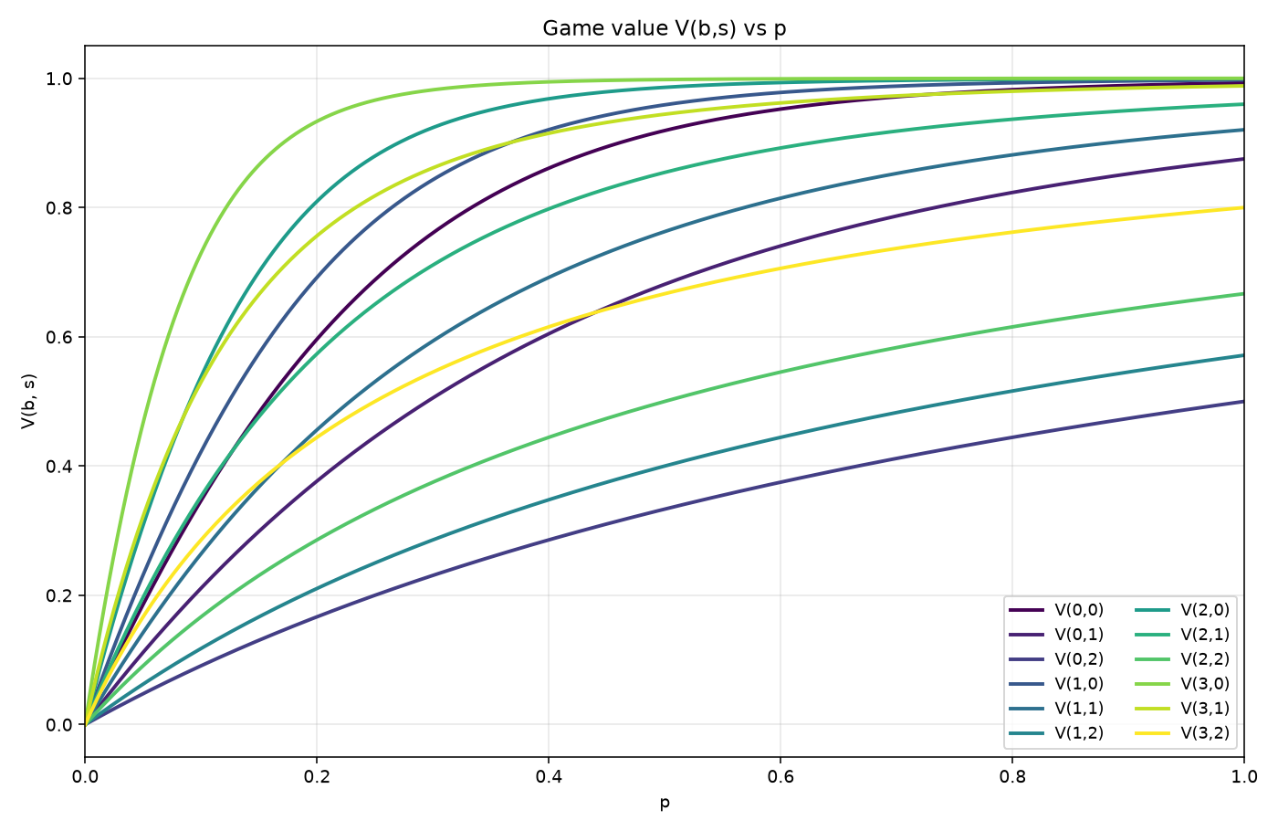
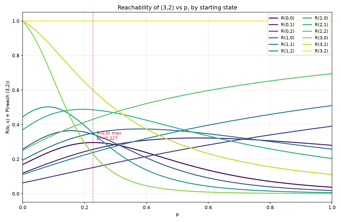
Look at that clean maximum for \(R(0,0)\)!
Black Box Search and Solving the Puzzle
Now we can calculate \(R(0,0)\) quickly for any value of \(p\) and can see in the plot above that \(R(0,0)\) has a clear single maximum in \([0,1]\). We can adapt Descartes’ Rule of Signs to rigorously prove that \(R(0,0)\) has a single maximum in \([0,1]\), but I will skip that.
Let’s calculate \(\operatorname*{arg\,max}\limits_{p \in [0,1]}\ R(0,0)\).
We will use golden section search, a blackbox (derivative free) optimization technique, because maximizing \(R(0,0)\) would involve computing the derivative of an insane rational polynomial in \(p\), which would cause a slew of precision issues that we don’t need to deal with.
This runs in less than a second. Here are our solutions to 10 decimal places:
\[\operatorname*{arg\,max}\limits_{p \in [0,1]}\ R(0,0) = 0.2269732325\] \[\operatorname*{max}\limits_{p \in [0,1]}\ R(0,0) = 0.2959679934\]Here is the search’s trace, in case you’re curious.
| N Evals | Lower Bound | Upper Bound | Best Guess max of R(0,0) |
|---|---|---|---|
| 0 | 0.000000000000 | 1.000000000000 | 0.247428935807 |
| 3 | 0.000000000000 | 0.618033988750 | 0.295748501269 |
| 4 | 0.000000000000 | 0.381966011250 | 0.295748501269 |
| 5 | 0.145898033750 | 0.381966011250 | 0.295748501269 |
| 6 | 0.145898033750 | 0.291796067501 | 0.295748501269 |
| 7 | 0.201626123751 | 0.291796067501 | 0.295748501269 |
| 8 | 0.201626123751 | 0.257354213752 | 0.295923558506 |
| 9 | 0.201626123751 | 0.236067977500 | 0.295923558506 |
| 10 | 0.214781741248 | 0.236067977500 | 0.295965502715 |
| 11 | 0.222912360003 | 0.236067977500 | 0.295965502715 |
| 12 | 0.222912360003 | 0.231042978759 | 0.295965543018 |
| 13 | 0.222912360003 | 0.227937358744 | 0.295965543018 |
| 14 | 0.224831738729 | 0.227937358744 | 0.295967861004 |
| 15 | 0.226017980019 | 0.227937358744 | 0.295967861004 |
| 16 | 0.226017980019 | 0.227204221308 | 0.295967861004 |
| 17 | 0.226471083872 | 0.227204221308 | 0.295967986922 |
| 18 | 0.226751117454 | 0.227204221308 | 0.295967986922 |
| 19 | 0.226751117454 | 0.227031151036 | 0.295967986922 |
| 20 | 0.226858080765 | 0.227031151036 | 0.295967993194 |
| 21 | 0.226924187726 | 0.227031151036 | 0.295967993194 |
| 22 | 0.226924187726 | 0.226990294687 | 0.295967993194 |
| 23 | 0.226949438338 | 0.226990294687 | 0.295967993369 |
| 24 | 0.226965044075 | 0.226990294687 | 0.295967993369 |
| 25 | 0.226965044075 | 0.226980649812 | 0.295967993369 |
| 26 | 0.226971004936 | 0.226980649812 | 0.295967993369 |
| 27 | 0.226971004936 | 0.226976965797 | 0.295967993374 |
| 28 | 0.226971004936 | 0.226974688951 | 0.295967993374 |
| 29 | 0.226972412104 | 0.226974688951 | 0.295967993374 |
| 30 | 0.226972412104 | 0.226973819273 | 0.295967993374 |
| 31 | 0.226972949595 | 0.226973819273 | 0.295967993374 |
| 32 | 0.226972949595 | 0.226973487085 | 0.295967993374 |
| 33 | 0.226973154898 | 0.226973487085 | 0.295967993374 |
| 34 | 0.226973154898 | 0.226973360201 | 0.295967993374 |
| 35 | 0.226973154898 | 0.226973281782 | 0.295967993374 |
| 36 | 0.226973203364 | 0.226973281782 | 0.295967993374 |
| 37 | 0.226973203364 | 0.226973251829 | 0.295967993374 |
| 38 | 0.226973221876 | 0.226973251829 | 0.295967993374 |
| 39 | 0.226973221876 | 0.226973240388 | 0.295967993374 |
| 40 | 0.226973228947 | 0.226973240388 | 0.295967993374 |
| 41 | 0.226973228947 | 0.226973236018 | 0.295967993374 |
| 42 | 0.226973231648 | 0.226973236018 | 0.295967993374 |
| 43 | 0.226973231648 | 0.226973234349 | 0.295967993374 |
| 44 | 0.226973231648 | 0.226973233317 | 0.295967993374 |
| 45 | 0.226973232285 | 0.226973233317 | 0.295967993374 |
| 46 | 0.226973232285 | 0.226973232923 | 0.295967993374 |
| 47 | 0.226973232285 | 0.226973232679 | 0.295967993374 |
| 48 | 0.226973232436 | 0.226973232679 | 0.295967993374 |
| 49 | 0.226973232436 | 0.226973232586 | 0.295967993374 |
| 50 | 0.226973232493 | 0.226973232586 | 0.295967993374 |
| 51 | 0.226973232493 | 0.226973232551 | 0.295967993374 |
| 52 | 0.226973232515 | 0.226973232551 | 0.295967993374 |
| 53 | 0.226973232529 | 0.226973232551 | 0.295967993374 |
| 54 | 0.226973232529 | 0.226973232542 | 0.295967993374 |